Improve the Performances

There are many ways to improve the performances of a simulation. This page provides a few tips to help achieving this goal.

Compilation Options

On Windows, the two following CMake variables may speed up the simulations:

• SOFA_ENABLE_FAST_MATH: Enable floating-point model to fast (theoretically faster but can bring unexpected results/bugs)
• SOFA_ENABLE_SIMD: Enable the use of SIMD instructions by the compiler (AVX/AVX2 for msvc).
• SOFA_ENABLE_LINK_TIME_OPTIMIZATION: Enable LTCG IN release mode (MSVC only for now) [Warning, use a lot of disk space!]

RunSofa

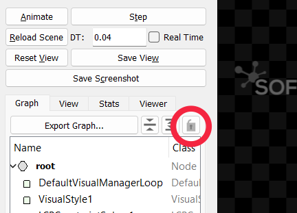
When running runSofa with the GUI, an option allows to update the visual representation of the scene graph if any change is detected (activated by default). It can affect badly the performances in high speed simulations. Disabling the option can help improving the performances: to do so, click on the lock icon as illustrated below.

Profile the Simulation

The first step toward better performances is to identify the bottleneck of the simulation. SOFA provides some tools to profile the simulation. See this page to learn how to use those tools. The principle is to measure the time taken by all major steps of the simulation. The timers are organized as a tree: a monitored step can call monitored substeps, making it a parent of the substeps.

Let us take the example of the caduceus demo, located in examples/Demos/caduceus.scn. The following image results from the profiling of one time step, measured in the GUI of runSofa.

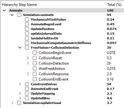
Two major steps can be identified:

1. FreeMotion+CollisionDetection
2. ConstraintSolver

Together, both steps account for 84% of the total computational time spent in the simulation step. In most simulation, those two steps will be the most time-consuming.

As the name suggests, the step FreeMotion+CollisionDetection gathers two substeps:

1. The collision detection
2. The free motion

These steps and their associated timers are specific to the FreeMotionAnimationLoop. Its particularity is that those two steps can be computed in parallel. It is the case in the example: collision detection takes 26% of the time. During that time, the free motion is computed in parallel. That is why the timer WaitFreeMotion is almost null. This parallelization is a possible solution to optimize the performances of this simulation. This parallelization is available because the computation of the free motion is also a time-consuming step of a simulation.

To summarize, the 3 major steps of a simulation, candidates for being a bottleneck, are:

1. Collision detection
2. Free motion
3. Constraint solving

In each of them, some substeps can be responsible of the bottleneck. The profiler helps identifying the one(s) . In the above example, the most time-consuming step is constraint solving, taking 54% of the time.

Collision Detection

If collision detection has been identified as a bottleneck, here are a few tips to improve the performances:

Asynchronous Free Motion

This tip requires to use a FreeMotionAnimationLoop.

The steps of collision detection and free motion are independent: they can be computed in parallel. The component FreeMotionAnimationLoop has boolean Data parallelCollisionDetectionAndFreeMotion to specify if both steps are computed in parallel or not. This optimization is the most effective when both steps takes about the same time. The total time of both steps computed in parallel will be the time taken by the most time-consuming one (plus the overhead due to parallelization).

Parallel Algorithms

There are high chances that a simulation uses BruteForceBroadPhase and BVHNarrowPhase. Multi-threaded versions of those two components are available in the MultiThreading plugin. Depending on the cases, the parallelization can help speeding up the collision detection phase. See details in the MultiThreading plugin dedicated page.

Free Motion

This step is computed in the FreeMotionAnimationLoop. However, there are also common steps with the DefaultAnimationLoop, such as the computation of the force, the matrix assembly and the solve of the linear system. Therefore, most of the tips of this section are also available for DefaultAnimationLoop.

The Choice of the Linear Solver

See this page for a description of the different types of linear solvers.

Iterative Solvers

The error reduces at each iteration of an iterative solver. Some of the parameters (e.g. iterations, tolerance and threshold in CGLinearSolver) controls when the solver stops its iterations. Less iterations means less computation, therefore faster simulations. Stopping too early can come at the price of too large error, and can even bring instabilities. With iterative solvers, finding an appropriate trade-off between accuracy and efficiency is key.

Matrix Assembly

When the linear solver assembles the system matrix in a compressed sparse row data structure, it is possible to use a matrix where the entries are blocs of 3×3. This is much faster to assemble. It is the most efficient when the simulation only involves 3 degrees of freedom per node (known as “Vec3d” in the SOFA template). The template parameter to use is CompressedRowSparseMatrixMat3x3d. Note that all solvers do not support this template parameter.

Matrix Assembly vs. Matrix Free

CGLinearSolver supports both strategies:

• GraphScattered is the template parameter for a matrix-free solver
• CompressedRowSparseMatrixd and CompressedRowSparseMatrixMat3x3d are template parameters for an assembled matrix

It is not always obvious which one is faster given the same number of iterations. However, it is easy to try both strategies: just change <CGLinearSolver template="GraphScattered"/> to <CGLinearSolver template="CompressedRowSparseMatrixMat3x3d"/>, and vice-versa, and compare the performances.

Asynchronous Linear Solver

SparseLDLSolver has an asynchronous equivalent (AsyncSparseLDLSolver), which the goal is to reduce the duration of the linear system solving. Computing asynchronously the LDL factorization of the matrix, this solver will however change the behavior of your simulation. Read more about it on the AsyncSparseLDLSolver page. In your scene, just replace <SparseLDLSolver/> by <AsyncSparseLDLSolver/>.

Parallel ODE Solving

This optimization requires to use a FreeMotionAnimationLoop. When multiple objects evolve in a simulation, SOFA supports the following configurations:

• There is a single ODE solver for all the objects.
• There are multiple ODE solvers, and each one can simulate one or multiple objects.

In the latter case, there are as many free motion computations as the number of ODE solvers in the scene. In this first step of the FreeMotionAnimationLoop, the free motion assumes that objects can have a “free” motion, thus ignoring possible interaction between objects. Therefore, the computation of the free motion of an object is independent from the others, and each ODE solve step can be trivially parallelized. The component FreeMotionAnimationLoop has boolean Data parallelODESolving to specify if both ODE solve steps are to be computed in parallel or not.

Finite Element Method

Several algorithms are available to simulate the same FEM model, so the simulation designer can choose depending on the constraints on the accuracy and speed of the simulation. For example, a component can have an alternative where the implementation uses approximations in order to speed up the computations. This is the case for the component TriangularFEMForceFieldOptim which is an alternative to TriangularFEMForceField. It has been measured that TriangularFEMForceFieldOptim is faster than TriangularFEMForceField. Similarly, the component FastTetrahedralCorotationalForceField is a faster alternative to TetrahedronFEMForceField, but without any compromise on the accuracy.

Rendering

• A data computeBoundingBox is available in all AnimationLoops. This data defines whether the global bounding box of the scene is computed at each time step. Setting this data to false will avoid the recomputation of the bounding box used for rendering, thus possibly saving computation time.

• Debug visualization can be very costly. For example, drawing thousands of tetrahedra is very time consuming. Draw only what you need.

Model Order Reduction

In SOFA, Model Order Reduction is a technique to reduce the computational complexity of a FEM simulation. It works with a premilinary step which precomputes deformation modes of an object. The modes are then used online, during a simulation, allowing to build and solve the same FEM problem in a reduced space, in order to dramatically increase the performances.

This technique is available in a plugin: https://github.com/SofaDefrost/ModelOrderReduction. Binaries are also available.

GPGPU

SOFA has a plugin allowing to compute some steps of the simulation on the GPU, based on CUDA. See this page. In most cases, the simulation is much faster when computed on the GPU, compared to the CPU version.